This blog is no longer updated (you can still read the previous posts).
Please visit:
https://thierrymoudiki.github.io/blog/
Thanks.
This blog is no longer updated (you can still read the previous posts).
Please visit:
https://thierrymoudiki.github.io/blog/
Thanks.
Filed under Uncategorized
Hi everyone! Best wishes for 2016!
In this post, I’ll show you how to use ESGtoolkit, for the simulation of Heston stochastic volatility model for stock prices.
If you’re interested in seeing other examples of use of ESGtoolkit, you can read these two posts: the Hull and White short rate model and the 2-factor Hull and White short rate model (G2++).
The Heston model was introduced by Steven Heston’s A closed-form solution for options with stochastic volatility with applications to bonds an currency options, 1993. For a fixed risk-free interest rate 
where 
In this model, under a certain probability, the stock price’s returns on very short periods of time of length 


On the other hand, 


By using this model, one can derive prices for European call options, as described in Calibrating Option Pricing Models with Heuristics. The authors provide a useful function called ‘callHestoncf’, which calculates these prices in R and Matlab.
Here’s the function’s description. I won’t reproduce the function here, please refer to the paper for details:
callHestoncf(S, X, tau, r, v0, vT, rho, k, sigma){
# S = Spot, X = Strike, tau = time to maturity
# r = risk-free rate, q = dividend yield
# v0 = initial variance, vT = long run variance (theta)
# rho = correlation, k = speed of mean reversion (kappa)
# sigma = volatility of volatility
}
Now, it’s time to use ESGtoolkit for Monte Carlo pricing. We are going to price 3 European Call options on 
rm(list=ls())
library(ESGtoolkit)

#Initial stock price
S0 <- 100
# Number of simulations (feel free to reduce this)
n <- 100000
# Sampling frequency
freq <- "monthly"
# volatility mean-reversion speed
kappa <- 0.003
# volatility of volatility
volvol <- 0.009
# Correlation between stoch. vol and spot prices
rho <- -0.5
# Initial variance
V0 <- 0.04
# long-term variance
theta <- 0.04
#Initial short rate
r0 <- 0.015

# Options maturities
horizon <- 15
# Options' exercise prices
strikes <- c(140, 100, 60)
For the simulation of the Heston model with ESGtoolkit, we first need to define how to make simulations of the terms
# Simulation of shocks with given correlation
set.seed(5) # reproducibility seed
shocks <- simshocks(n =  n,
horizon =  horizon,
frequency =  freq,
method = "anti",
family = 1, par =  rho)
This function provides a list with 2 components, each containing simulated random gaussian increments. Both of these components will be useful for the simulation of 
#  Stochastic volatility  simulation
sim.vol <- simdiff(n =  n, horizon =  horizon,
frequency =  freq, model = "CIR", x0 =  V0,
theta1 =  kappa*theta, theta2 =  kappa,
theta3 =  volvol, eps =  shocks[[1]])

# Stock prices simulation
sim.price <- simdiff(n = n, horizon = horizon,
frequency = freq, model = "GBM", x0 = S0,
theta1 = r0, theta2 = sqrt(sim.vol),
eps = shocks[[2]])
We are now able to calculate options prices, with the 3 different
exercise prices. You’ll need to have imported ‘callHestoncf’, for this piece of code to work.
# Stock price at maturity (15 years)
S_T <- sim.price[nrow(sim.price), ]

### Monte Carlo prices
#### Estimated Monte Carlo price
discounted.payoff <- function(x)
{
(S_T - x)*(S_T - x > 0)*exp(-r0*horizon)
}
mcprices <- sapply(strikes, function(x)
mean(discounted.payoff(x)))

#### 95% Confidence interval around the estimation
mcprices95 <- sapply(strikes,  function(x)
t.test(discounted.payoff(x),
conf.level = 0.95)$conf.int)

#### 'Analytical' prices given by 'callHestoncf'
pricesAnalytic <- sapply(strikes, function(x)
callHestoncf(S = S0, X = x, tau = horizon,
r = r0, q = 0, v0 = V0, vT = theta,
rho = rho, k = kappa, sigma = volvol))

results <- data.frame(cbind(strikes, mcprices,
t(mcprices95), pricesAnalytic))
colnames(results) <- c("strikes", "mcprices", "lower95",
"upper95", "pricesAnalytic")

print(results)

strikes mcprices  lower95  upper95 pricesAnalytic
1     140 25.59181 25.18569 25.99793         25.96174
2     100 37.78455 37.32418 38.24493         38.17851
3      60 56.53187 56.02380 57.03995         56.91809
From these results, we see that the Monte Carlo prices for the 3 options are
fairly close to the price calculated by using the function ‘callHestoncf’
(uses directly formulas for the prices calculation). The 95% confidence
interval contains the theoretical price. Do not hesitate to change the seed,
and re-run the previous code.
Below are the option prices, as functions of the number of simulations.
The theoretical price calculated by ‘callHestoncf’ is drawn in blue,
the average Monte Carlo price in red, and the shaded region represents
the 95% confidence interval around the mean (the Monte Carlo price).
Filed under ESGtoolkit, R stuff
In this post, I use R packages RQuantLib and ESGtoolkit for the calibration and simulation of the famous Hull and White short-rate model.
QuantLib is an open source C++ library for quantitative analysis, modeling, trading, and risk management of financial assets. RQuantLib is built upon it, providing R users with an interface to the library .
ESGtoolkit provides tools for building Economic Scenarios Generators (ESG) for Insurance. The package is primarily built for research purpose, and comes with no warranty. For an introduction to ESGtoolkit, you can read this slideshare, or this blog post. A development version of the package is available on Github with, I must admit, only 2 or 3 commits for now.
The Hull and White (1994) model was proposed to address Vasicek’s model poor fitting of the initial term structure of interest rates. The model is defined as:
Where 


An alternative and convenient representation of the model is:
where
and 

In insurance market consistent pricing, the model is often calibrated to swaptions, as there are no market prices for embedded options and guarantees.
Two parameters
It’s worth mentioning that the yield curve bootstrapping procedure currently implemented in RQuantLib, makes the implicit assumption that LIBOR is a good proxy for risk-free rates, and collateral doesn’t matter. These assumptions are still widely used in insurance, along with simple (parallel) adjustments for credit/liquidity risks, but were abandoned by markets after the 2007 subprime crisis.
For more details on the new multiple-curve approach, see for example http://papers.ssrn.com/sol3/papers.cfm?abstract_id=2219548. In this paper, the authors introduce a multiple-curve bootstrapping procedure, available in QuantLib.
# Cleaning the workspace
rm(list=ls())
# RQuantLib loading
suppressPackageStartupMessages(library(RQuantLib))
# ESGtoolkit loading
suppressPackageStartupMessages(library(ESGtoolkit))
# Frequency of simulation and interpolation
freq <- "monthly"
delta_t <- 1/12
# This data is taken from sample code shipped with QuantLib 0.3.10.
params <- list(tradeDate=as.Date('2002-2-15'),
settleDate=as.Date('2002-2-19'),
payFixed=TRUE,
dt=delta_t,
strike=.06,
method="HWAnalytic",
interpWhat="zero",
interpHow= "spline")
# Market data used to construct the term structure of interest rates
# Deposits and swaps
tsQuotes <- list(d1w =0.0382,
d1m =0.0372,
d3m = 0.0363,
d6m = 0.0353,
d9m = 0.0348,
d1y = 0.0345,
s2y = 0.037125,
s3y =0.0398,
s5y =0.0443,
s10y =0.05165,
s15y =0.055175)
# Swaption volatility matrix with corresponding maturities and tenors
swaptionMaturities <- c(1,2,3,4,5)
swapTenors <- c(1,2,3,4,5)
volMatrix <- matrix(
c(0.1490, 0.1340, 0.1228, 0.1189, 0.1148,
0.1290, 0.1201, 0.1146, 0.1108, 0.1040,
0.1149, 0.1112, 0.1070, 0.1010, 0.0957,
0.1047, 0.1021, 0.0980, 0.0951, 0.1270,
0.1000, 0.0950, 0.0900, 0.1230, 0.1160),
ncol=5, byrow=TRUE)
# Pricing the Bermudan swaptions
pricing <- RQuantLib::BermudanSwaption(params, tsQuotes,
swaptionMaturities, swapTenors, volMatrix)
summary(pricing)
# Constructing the spot term structure of interest rates
# based on input market data
times <- seq(from = delta_t, to = 5, by = delta_t)
curves <- RQuantLib::DiscountCurve(params, tsQuotes, times)
maturities <- curves$times
marketzerorates <- curves$zerorates
marketprices <- curves$discounts
############# Hull-White short-rates simulaton
# Horizon, number of simulations, frequency
horizon <- 5 # I take horizon = 5 because of swaptions maturities
nb.sims <- 10000
# Calibrated Hull-White parameters from RQuantLib
a <- pricing$a
sigma <- pricing$sigma
# Simulation of gaussian shocks with ESGtoolkit
set.seed(4)
eps <- ESGtoolkit::simshocks(n = nb.sims, horizon = horizon,
frequency = freq)
# Simulation of the factor x with ESGtoolkit
x <- ESGtoolkit::simdiff(n = nb.sims, horizon = horizon,
frequency = freq,
model = "OU",
x0 = 0, theta1 = 0,
theta2 = a,
theta3 = sigma,
eps = eps)
# I use RQuantlib's forward rates. With the low monthly frequency,
# I consider them as being instantaneous forward rates
fwdrates <- ts(replicate(nb.sims, curves$forwards),
start = start(x),
deltat = deltat(x))
# alpha
t.out <- seq(from = 0, to = horizon, by = delta_t)
param.alpha <- ts(replicate(nb.sims, 0.5*(sigma^2)*(1 - exp(-a*t.out))^2/(a^2)),
start = start(x), deltat = deltat(x))
alpha <- fwdrates + param.alpha
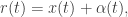
# The short-rate
r <- x + alpha
# Stochastic discount factors (numerical integration currently is very basic)
Dt <- ESGtoolkit::esgdiscountfactor(r = r, X = 1)
# Monte Carlo prices and zero rates deduced from stochastic discount factors
montecarloprices <- rowMeans(Dt)
montecarlozerorates <- -log(montecarloprices)/maturities # RQuantLib uses continuous compounding
# Confidence interval for the difference between market and monte carlo prices
conf.int <- t(apply((Dt - marketprices)[-1, ], 1, function(x) t.test(x)$conf.int))
# Viz
par(mfrow = c(2, 2))
# short-rate quantiles
ESGtoolkit::esgplotbands(r, xlab = "maturities", ylab = "short-rate quantiles",
main = "short-rate quantiles")
# monte carlo vs market zero rates
plot(maturities, montecarlozerorates, type='l', col = 'blue', lwd = 3,
main = "monte carlo vs market \n zero rates")
points(maturities, marketzerorates, col = 'red')
# monte carlo vs market zero-coupon prices
plot(maturities, montecarloprices, type ='l', col = 'blue', lwd = 3,
main = "monte carlo vs market \n zero-coupon prices")
points(maturities, marketprices, col = 'red')
# confidence interval for the price difference
matplot(maturities[-1], conf.int, type = 'l',
main = "confidence interval \n for the price difference")

Filed under R stuff
The whole post can be found here on RPubs, as (according to me !) this website provides a nice display for R code, figures and LaTeX formulas. Plus, you can publish directly on Rpubs, simply by using Markdown within RStudio.
Concerning the post content, it’s worth saying that there also a numerical integration error, induced by the calculation of discount factors.
For more ressources on ESGtoolkit, you can read these slides of a talk that I gave last month at Institut de Sciences Financières et d’Assurances (Université Lyon 1), and the package vignette.
Please, cite the package whenever you use it, according to citation(“ESGtoolkit”). And do not hesitate to report bugs or send features request 😉
Filed under Conference Talks, R stuff